import os
import feather
import pandas as pd
import numpy as np
import umap
import matplotlib.pyplot as plt
import seaborn as sns
from sklearn.pipeline import Pipeline
from sklearn.preprocessing import PowerTransformer
from sklearn.model_selection import RepeatedStratifiedKFold, cross_val_score, GridSearchCV
from sklearn.linear_model import LogisticRegression
from sklearn.metrics import roc_curve, plot_roc_curve, roc_auc_score

from sle.modeling import generate_data, prep_data, eval_model, calc_roc_cv, plot_roc_cv
from sle.penalization import regularization_range, choose_C
%load_ext autoreload
%autoreload 2Main Results
Citation
This notebook reproduces results reported in the following paper:
Brunekreef TE, Reteig LC, Limper M, Haitjema S, Dias J, Mathsson-Alm L, van Laar JM, Otten HG. Microarray analysis of autoantibodies can identify future Systemic Lupus Erythematosus patients. Human Immunology. 2022 Apr 11. doi:10.1016/j.humimm.2022.03.010
Setup
Running the code without the original data
If you want to run the code but don’t have access to the data, run the following instead to generate some synthetic data:
data_all = generate_data('imid')
X_test_df = generate_data('rest')
Code for loading original data
data_dir = os.path.join('..', 'data', 'processed')
data_all = feather.read_dataframe(os.path.join(data_dir, 'imid.feather'))
X_test_df = feather.read_dataframe(os.path.join(data_dir,'rest.feather'))
Projection
See the projection.ipynb notebook for extended results and analyses
trf = PowerTransformer(method='box-cox')df_combined = pd.concat([data_all, X_test_df[X_test_df.Class.isin(['preSLE', 'rest_large'])]])
df_combined['Class'] = pd.Categorical(df_combined.Class, categories = ['SLE','IMID','nonIMID','rest_large','BBD','preSLE']) # order for plotting: largest groups first
df_combined.sort_values(by='Class', inplace=True)
X_combined = np.array(df_combined.loc[:, ~df_combined.columns.isin(["Arthritis","Pleurisy","Pericarditis","Nefritis"] + ['Class'] + ['dsDNA1'])])
X_combined_scaled = trf.fit_transform(X_combined+1)X_combined.shape(1887, 57)df_combined.Class.value_counts()SLE 483
rest_large 462
BBD 361
IMID 346
nonIMID 218
preSLE 17
Name: Class, dtype: int64umap_obj = umap.UMAP(random_state=42)
Y_umap_combined = umap_obj.fit_transform(X_combined_scaled)df_combined['umap_1'] = Y_umap_combined[:,0]
df_combined['umap_2'] = Y_umap_combined[:,1]Figure 1
with sns.plotting_context("paper"):
    sns.set(font="Arial")
    sns.set_style('white')
    f, ax = plt.subplots(figsize=(5.5, 5.5))
    g = sns.scatterplot(x='umap_1',y='umap_2',
                    hue='Class', style='Class', size='Class',
                    markers = {"SLE": "o", "rest_large": "o", "BBD": "o", "IMID": "o", "nonIMID": "o", "preSLE": "o"},
                    sizes = {"SLE": 20, "rest_large": 20, "BBD": 20, "IMID": 20, "nonIMID": 20, "preSLE": 20},
                    palette={"SLE": '#0072B2', "rest_large": '#D55E00', "BBD": '#CC79A7', "IMID": '#009E73', "nonIMID": '#E69F00', "preSLE": '#000000'},
                    alpha=.7,
                    data=df_combined,
                    ax=ax)
    legend = ax.legend(frameon=False, loc = 'upper left', bbox_to_anchor=(0,1.05))
    ax.set_xlabel('Dimension 1'); ax.set_ylabel('Dimension 2');
    ax.set_ylim(-6,0)
    new_labels = ['','SLE','IMID','Non-IMID','Rest','BBD','Pre-SLE']; # remove legend title and change group spelling
    for t, l in zip(legend.texts, new_labels): t.set_text(l)
    sns.despine(fig=f,ax=ax)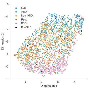
Prediction models
X_nonIMID, y_nonIMID = prep_data(data_all, 'SLE', 'nonIMID', drop_cols = ["Arthritis","Pleurisy","Pericarditis","Nefritis","dsDNA1"])
dsDNA_nonIMID = X_nonIMID.dsDNA2.values.reshape(-1,1)
clf = LogisticRegression(penalty = 'none', max_iter = 10000)cv = RepeatedStratifiedKFold(n_splits=5, n_repeats=5, random_state=40)SLE vs. non-IMID
See the SLE Versus nonIMID.ipynb notebook for extended analyses and results
Logistic regression: Only dsDNA from microarray
lr_dsDNA_nonIMID = clf.fit(dsDNA_nonIMID, y_nonIMID)np.mean(cross_val_score(clf, dsDNA_nonIMID, y_nonIMID, cv=cv, scoring = 'roc_auc'))0.8006217102395325Logistic regression: Whole microarray
Xp1_nonIMID = X_nonIMID + 1 # Some < 0 values > -1. Because negative fluorescence isn't possible, and Box-Cox requires strictly positive values, add ofsetpipe_trf = Pipeline([
('transform', trf),
('clf', clf)])np.mean(cross_val_score(pipe_trf, Xp1_nonIMID, y_nonIMID, cv=cv, scoring = 'roc_auc'))0.8337294463757692LASSO
clf_lasso = LogisticRegression(penalty='l1', max_iter = 10000, solver = 'liblinear')K = 100
lambda_min, lambda_max = regularization_range(Xp1_nonIMID,y_nonIMID,trf)
Cs_lasso_nonIMID = np.logspace(np.log10(1/lambda_min),np.log10(1/lambda_max), K)
pipe = Pipeline([
('trf', trf),
('clf', clf_lasso)
])
params = [{
"clf__C": Cs_lasso_nonIMID
}]
lasso_nonIMID = GridSearchCV(pipe, params, cv = cv, scoring = 'roc_auc', refit=choose_C)%%time
lasso_nonIMID.fit(Xp1_nonIMID,y_nonIMID)CPU times: user 3min 33s, sys: 64.1 ms, total: 3min 33s
Wall time: 3min 33sGridSearchCV(cv=RepeatedStratifiedKFold(n_repeats=5, n_splits=5, random_state=40),
estimator=Pipeline(steps=[('trf',
PowerTransformer(method='box-cox')),
('clf',
LogisticRegression(max_iter=10000,
penalty='l1',
solver='liblinear'))]),
param_grid=[{'clf__C': array([6.52012573, 6.08069108, 5.67087285, 5.288675 , 4.932236 ,
4.5998198 , 4.28980735, 4.00068869, 3.73105566, 3...
0.04932236, 0.0459982 , 0.04289807, 0.04000689, 0.03731056,
0.03479595, 0.03245082, 0.03026374, 0.02822407, 0.02632186,
0.02454785, 0.02289341, 0.02135047, 0.01991152, 0.01856955,
0.01731803, 0.01615085, 0.01506234, 0.01404719, 0.01310045,
0.01221753, 0.0113941 , 0.01062618, 0.00991001, 0.00924211,
0.00861922, 0.00803832, 0.00749656, 0.00699132, 0.00652013])}],
refit=<function choose_C at 0x7f80d43e74d0>, scoring='roc_auc')Best model AUC:
lasso_nonIMID.cv_results_['mean_test_score'].max()0.8373932541974528AUC with lambda selected through 1 SE rule:
lasso_nonIMID.cv_results_['mean_test_score'][lasso_nonIMID.best_index_]0.8334140652811983Number of non-zero coefficients in this model:
coefs_final_nonimid = (pd.Series(lasso_nonIMID.best_estimator_.named_steps.clf.coef_.squeeze(),
                                 index = X_nonIMID.columns)[lambda x: x!=0].sort_values())
len(coefs_final_nonimid)29Figure 2 (top panel)
sns.reset_defaults()
with sns.plotting_context("paper"):
    fig, ax = plt.subplots(figsize=(4.5, 4.5))
    tprs, aucs = calc_roc_cv(lasso_nonIMID.best_estimator_,cv,Xp1_nonIMID,y_nonIMID)
    fig, ax = plot_roc_cv(tprs, aucs, fig, ax, fig_title='SLE vs. non-IMID', line_color='#E69F00', legend_label='LASSO')
    tprs, aucs = calc_roc_cv(lr_dsDNA_nonIMID,cv,dsDNA_nonIMID,y_nonIMID)
    fig, ax = plot_roc_cv(tprs, aucs, fig, ax, reuse=True, line_color='gray', legend_label='dsDNA (from chip) only')
    sns.despine(fig=fig,ax=ax, trim=True)
    plt.legend(frameon=False)
    plt.show()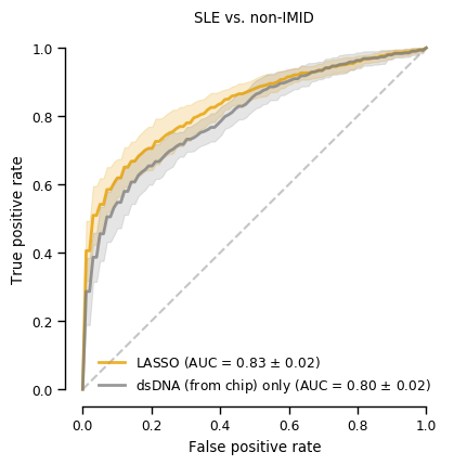
Supplemental Figure 1a
sns.reset_defaults()
pal = sns.diverging_palette(250, 15, s=75, l=40, center="dark", as_cmap=True)
with sns.plotting_context("paper"):
    with sns.axes_style("whitegrid"):
        fig, ax = plt.subplots(figsize=(2.5, 5))
        g = sns.scatterplot(y=coefs_final_nonimid.index, x=coefs_final_nonimid.values,
                            hue=coefs_final_nonimid.values, palette=pal, legend=False)
        ax.set(title='SLE vs.non-IMID',
               xticks=np.linspace(-1.0,1.0,5), xlim=[-1.2,1.2], xlabel=r'$\beta$')
        sns.despine(fig=fig,ax=ax, left=True, bottom=True)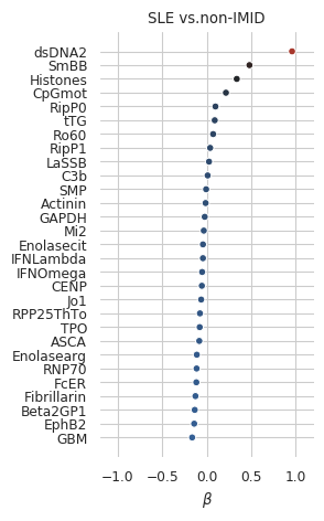
SLE vs. BBD (Blood Bank Donors)
See the SLE Versus BBD.ipynb notebook for extended analyses and results
Logistic regression: Only one feature
X, y = prep_data(data_all, 'SLE', 'BBD', drop_cols = ["Arthritis","Pleurisy","Pericarditis","Nefritis"] + ["dsDNA1"])
dsDNA = X.dsDNA2.values.reshape(-1,1)
Ro60 = X.Ro60.values.reshape(-1,1)
dsDNA from microarray
lr_dsDNA = clf.fit(dsDNA, y)np.mean(cross_val_score(clf, dsDNA, y, cv=cv, scoring = 'roc_auc'))0.7956906204723647Ro60 from microarray
np.mean(cross_val_score(clf, Ro60, y, cv=cv, scoring = 'roc_auc'))0.8980197798817389LASSO
Xp1 = X + 1 # Some values are between -1 and 0. Because negative fluorescence isn't possible, and Box-Cox requires strictly positive values, add ofsetlambda_min, lambda_max = regularization_range(Xp1,y,trf)K = 100
Cs_lasso = np.logspace(np.log10(1/lambda_min),np.log10(1/lambda_max), K)
pipe = Pipeline([
('trf', trf),
('clf', clf_lasso)
])
params = [{
"clf__C": Cs_lasso
}]
search_lasso = GridSearchCV(pipe, params, cv = cv, scoring = 'roc_auc', refit=choose_C)%%time
search_lasso.fit(Xp1,y)CPU times: user 9min 2s, sys: 17min 14s, total: 26min 16s
Wall time: 4min 36sGridSearchCV(cv=RepeatedStratifiedKFold(n_repeats=5, n_splits=5, random_state=40),
estimator=Pipeline(steps=[('trf',
PowerTransformer(method='box-cox')),
('clf',
LogisticRegression(max_iter=10000,
penalty='l1',
solver='liblinear'))]),
param_grid=[{'clf__C': array([3.42342671, 3.19269921, 2.97752197, 2.77684695, 2.58969676,
2.41515987, 2.25238618, 2.10058289, 1.95901...
0.02589697, 0.0241516 , 0.02252386, 0.02100583, 0.01959011,
0.0182698 , 0.01703848, 0.01589014, 0.0148192 , 0.01382043,
0.01288898, 0.01202031, 0.01121018, 0.01045465, 0.00975004,
0.00909292, 0.00848009, 0.00790856, 0.00737555, 0.00687846,
0.00641488, 0.00598254, 0.00557933, 0.0052033 , 0.00485262,
0.00452557, 0.00422056, 0.00393611, 0.00367083, 0.00342343])}],
refit=<function choose_C at 0x7f80d43e74d0>, scoring='roc_auc')Best model AUC:
search_lasso.cv_results_['mean_test_score'].max()0.9829972773711079AUC with lambda selected through 1 SE rule:
search_lasso.cv_results_['mean_test_score'][search_lasso.best_index_]0.9813334155499589Number of non-zero coefficients in this model:
coefs_final = (pd.Series(search_lasso.best_estimator_.named_steps.clf.coef_.squeeze(),
                                 index = X_nonIMID.columns)[lambda x: x!=0].sort_values())
len(coefs_final)15Figure 2 (bottom panel)
sns.reset_defaults()
with sns.plotting_context("paper"):
    fig, ax = plt.subplots(figsize=(4.5, 4.5))
    tprs, aucs = calc_roc_cv(search_lasso.best_estimator_,cv,Xp1,y)
    fig, ax = plot_roc_cv(tprs, aucs, fig, ax, fig_title='SLE vs. BBD', line_color='#CC79A7', legend_label='LASSO')
    tprs, aucs = calc_roc_cv(lr_dsDNA,cv,dsDNA,y)
    fig, ax = plot_roc_cv(tprs, aucs, fig, ax, reuse=True, line_color='gray', legend_label='dsDNA only')
    sns.despine(fig=fig,ax=ax, trim=True)
    plt.legend(frameon=False)
    plt.show()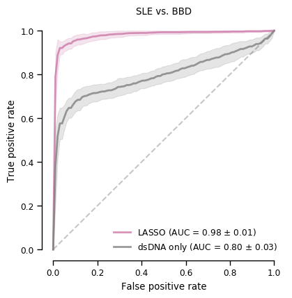
Supplemental Figure 1b
sns.reset_defaults()
pal = sns.diverging_palette(250, 15, s=75, l=40, center="dark", as_cmap=True)
with sns.plotting_context("paper"):
    with sns.axes_style("whitegrid"):
        fig, ax = plt.subplots(figsize=(2.5, 2.5))
        g = sns.scatterplot(y=coefs_final.index, x=coefs_final.values,
                            hue=coefs_final.values, palette=pal, legend=False)
        ax.set(title='SLE vs. BBD',
               xticks=np.linspace(-1.0,1.0,5), xlim=[-1.2,1.2], xlabel=r'$\beta$')
        sns.despine(fig=fig,ax=ax, left=True, bottom=True)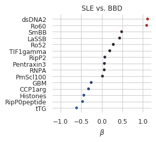
Prediction of the development of SLE
ROC AUC of SLE vs. BBD model
X_test, y_test = prep_data(X_test_df, 'preSLE', 'rest_large', ["Arthritis","Pleurisy","Pericarditis","Nefritis"] + ["dsDNA1"])
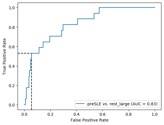
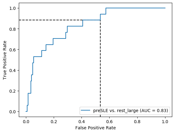
roc_auc_score(y_test, search_lasso.predict_proba(X_test+1)[:,1])0.5679908326967151Figure 3
X_test, y_test = prep_data(X_test_df, 'preSLE', 'rest_large', ["Arthritis","Pleurisy","Pericarditis","Nefritis"] + ["dsDNA1"])
# ROC curve
threshold1=0.5
threshold2=0.84
fpr, tpr, thresholds = roc_curve(y_test, lasso_nonIMID.predict_proba(X_test+1)[:,1])
thr_idx1 = (np.abs(thresholds - threshold1)).argmin() # find index of value closest to chosen threshold
thr_idx2 = (np.abs(thresholds - threshold2)).argmin() # find index of value closest to chosen threshold
sns.reset_defaults()
with sns.plotting_context("paper"):
    fig, ax = plt.subplots(figsize=(4.5, 4.5))
    ax.plot([0, 1], [0, 1], linestyle='--', lw=1.5, color='k', alpha=.25)
    ax.set(title="Pre-SLE vs. Rest",
           xlim=[-0.05, 1.05], xlabel='False positive rate',
           ylim=[-0.05, 1.05], ylabel='True positive rate')
    ymin, ymax = ax.get_ylim(); xmin, xmax = ax.get_xlim()
    plt.vlines(x=fpr[thr_idx1], ymin=ymin, ymax=tpr[thr_idx1], color='k', alpha=.6, linestyle='--', axes=ax) # plot line for fpr at threshold
    plt.hlines(y=tpr[thr_idx1], xmin=xmin, xmax=fpr[thr_idx1], color='k', alpha=.6, linestyle='--', axes=ax) # plot line for tpr at threshold
    plt.vlines(x=fpr[thr_idx2], ymin=ymin, ymax=tpr[thr_idx2], color='k', alpha=.6, linestyle='--', axes=ax) # plot line for fpr at threshold
    plt.hlines(y=tpr[thr_idx2], xmin=xmin, xmax=fpr[thr_idx2], color='k', alpha=.6,  linestyle='--', axes=ax) # plot line for tpr at threshold
    plot_roc_curve(lasso_nonIMID, X_test+1, y_test, name = "LASSO", ax=ax, color='#D55E00', lw=2, alpha=.8)
    plt.text(0.56,0.81, '1', fontsize='large')
    plt.text(0.08,0.45, '2', fontsize='large')
    sns.despine(fig=fig,ax=ax, trim=True)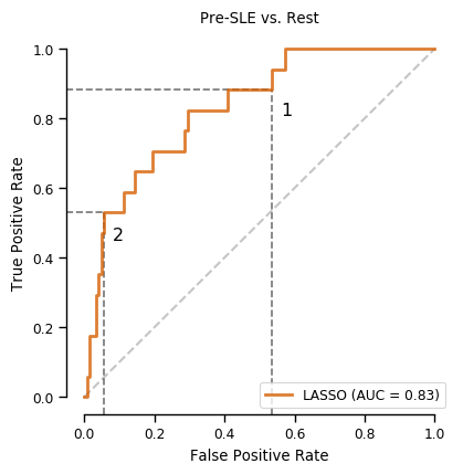
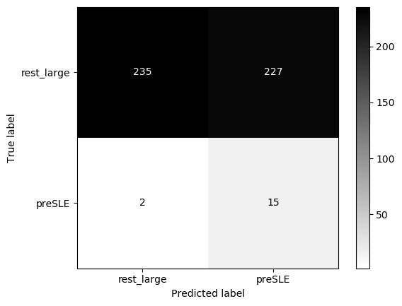
Classification
X_test, y_test = prep_data(X_test_df, 'preSLE', 'rest_large', ["Arthritis","Pleurisy","Pericarditis","Nefritis"] + ["dsDNA1"])
eval_model(lasso_nonIMID, X_test+1, y_test, 'preSLE', 'rest_large')
Threshold for classification: 0.5
precision recall f1-score support
rest_large 0.99 0.51 0.67 462
preSLE 0.06 0.88 0.12 17
accuracy 0.52 479
macro avg 0.53 0.70 0.39 479
weighted avg 0.96 0.52 0.65 479
N.B.: "recall" = sensitivity for the group in this row (e.g. preSLE); specificity for the other group (rest_large)
N.B.: "precision" = PPV for the group in this row (e.g. preSLE); NPV for the other group (rest_large)
X_test, y_test = prep_data(X_test_df, 'preSLE', 'rest_large', ["Arthritis","Pleurisy","Pericarditis","Nefritis"] + ["dsDNA1"])
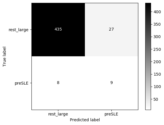
eval_model(lasso_nonIMID, X_test+1, y_test, 'preSLE', 'rest_large', threshold=0.84)Threshold for classification: 0.84
precision recall f1-score support
rest_large 0.98 0.94 0.96 462
preSLE 0.25 0.53 0.34 17
accuracy 0.93 479
macro avg 0.62 0.74 0.65 479
weighted avg 0.96 0.93 0.94 479
N.B.: "recall" = sensitivity for the group in this row (e.g. preSLE); specificity for the other group (rest_large)
N.B.: "precision" = PPV for the group in this row (e.g. preSLE); NPV for the other group (rest_large)